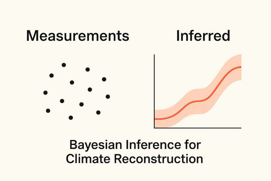
Challenge in Bayesian inference for climate reconstruction
Background
Paleoclimate reconstruction aims at estimating how Earth’s climate, in particular surface temperature, has changed over timescales that extend far beyond the period covered by instrumental observations. Since direct measurements are only available for roughly the last 150 years, information about earlier climate states has to be obtained from indirect observations, so-called proxy data. Typical examples include isotopic compositions from ice cores, annual growth layers in tree rings, chemical signatures in marine sediments, or coral records. These proxies do not measure temperature directly, but are influenced by it through physical, chemical, or biological processes. As a result, paleoclimate data are heterogeneous, noisy, irregular in time, and spatially sparse.
The reconstruction problem then consists in inferring past temperatures from these indirect observations. This requires assumptions about how proxy records relate to climate variables and about the structure of uncertainties in the data. Because proxy coverage is incomplete and the proxy–temperature relationship is imperfect, the resulting reconstructions are necessarily uncertain. From a methodological point of view, this setting is closely related to standard inference problems in statistics and data analysis: estimating latent variables from noisy observations, combining multiple data sources, and working with time series and spatial data. Corresponding tools range from relatively simple regression approaches to more complex probabilistic and machine-learning-based methods.
In this challenge, we do not try to actually solve a surface temperature reconstruction problem, as in paleo-climate reconstruction. Instead, we have a look at a simplified Bayesian inference task that contains a lot of the technicalities that a PhD student in the field will be exposed to. The intention is to gather a first orientation on the expected work that will be conducted during the PhD thesis.
The challenge: Bayesian Inference for a heat distribution problem
This task is concerned with the investigation of an inverse problem in the context of the heat distribution, expressed by the Poisson equation on the domain Ω=[0,1]2. In particular, we assume to have boundary conditions for three boundaries given, as well as selected measurements of the solution, i.e. temperatures inside the domain, and aim at recovering the fourth boundary condition from that information.
The Poisson problem
As said before, we consider the Poisson problem on the unit square. In this setting we cool three sides, i.e. we fix a Dirichlet boundary condition with a constant temperature of zero degrees on the bottom, right-hand side and the top. On the left boundary, an unknown heating is applied, which is a not necessarily constant, non-zero Dirichlet boundary condition. We formalize the problem as
$$
\begin{align}
\nabla^2 u(x,y) &= 0, && (x,y)\in (0,1)^2 \\
u(x,0) &= 0, && x\in(0,1) \\
u(x,1) &= 0, && x\in(0,1) \\
u(1,y) &= 0, && y\in [0,1] \\
u(0,y) &= f(y), && y\in[0,1]
\end{align}
$$
Here \( f:[0,1] \to \mathbb{R} \) models the unknown “heating” on the left boundary of the square. We want to infer the left boundary condition \( f(y) = u(0,y),\ y\in[0,1] \). The above problem can be solved numerically using finite differences (FD) with grid size \( h \).
Boundary representation
We assume that the unknown boundary condition can be approximated as a linear combination of \( k \) Gaussian radial basis functions, centered at locations \( \{y_1^{bc},\ldots,y_k^{bc}\} \), i.e.
$$
f(y) = \sum_{j=1}^k \alpha_j \, \phi(y, y_j^{bc}),
$$
where \( \alpha:=(\alpha_1, …, \alpha_k)\in\mathbb{R}^k \) are coefficients and \( \phi: [0,1]\times[0,1] \to \mathbb{R} \) is the (1D) Gaussian radial basis function (RBF) given by
$$
\phi(y,y^\prime) = \exp\left(-\frac{(y-y^\prime)^2}{2\ell^2}\right).
$$
Collecting measurements
We are given \( m \) measurement locations \( \left\{ \left( x_i^{\text{obs}}, y_i^{\text{obs}} \right) \right\}_{i=1}^m \). For these, we solve the Poisson problem, for the given boundary \( f \). Note that the above boundary representation allows us to express the currently selected boundary condition \( f \) just by the coefficients \( \alpha \). Hence if we express \(f\) via the above basis expansion, then the solution of the Poisson equation evaluated at coordinate \( (x,y) \) is given by $$u[\alpha](x,y).$$ We can then collect \( m \) exact (point!) evaluations as a vector
$$
\begin{pmatrix}
u[\alpha](x_1^{\text{obs}}, y_1^{\text{obs}})\\
\vdots \\
u[\alpha](x_m^{\text{obs}}, y_m^{\text{obs}})
\end{pmatrix}
$$
In practice, no technical measurement device is able to provide actual point measurements. It rather collects measurement information that is “smeared out” around the actual point of measurement. We do the same, here, and use “mollified” point evaluations, where we apply a “smearing” with a radius of \( \tau \). Hence our measurements are no longer \( u[\alpha]\) but \( u_\tau[\alpha]\).
More formally, we thereby can now introduce the forward map \( \Phi: \mathbb{R}^k \to \mathbb{R}^m, \ \alpha \mapsto \Phi(\alpha) \) with
$$
\Phi(\alpha) :=
\begin{pmatrix}
u_{\tau}[\alpha](x_1^{\text{obs}}, y_1^{\text{obs}})\\
\vdots \\
u_{\tau}[\alpha](x_m^{\text{obs}}, y_m^{\text{obs}})
\end{pmatrix}
$$
This is nothing else than the just introduced (mollified version) of evaluations of the solution in \( m \) observation points, if we fix the coefficient vector \( \alpha \) describing the boundary condition \( f \).
Data
Participants are given “realistic” measurements for an unknown boundary condition \( f \), i.e. unknown \( \alpha \), in the \( \texttt{measurements.npz} \) file. The data \( d = (d_1,\ldots,d_m) \) comes from noisy measurements, i.e. it is generated as
$$
d = \Phi(\alpha) + \sigma_\varepsilon,
$$
where the noise \( \sigma_\varepsilon \) follows some zero mean distribution.
The file contains
- the measurement locations \( \left\{ \left( x_i^{\text{obs}}, y_i^{\text{obs}} \right) \right\}_{i=1}^m \) and “realistic” measurements \( d \),
- an estimate to the noise level of the measured data (which can be helpful for the inference),
- the grid points of the applied finite difference discretization, and
- reference samples from the true (to be found) boundary \( f(y) \). These are for comparison purposes only!
There exists a helper function “load_data”, which loads the measurement file and returns the data appropriately. (Please note the documentation of that helper function for further details.)
Bayesian formulation of the inference task
The objective is now to infer the unknown coefficient vector \( \alpha \) from the given data \( d \).
In the Bayesian framework, the coefficient vector \( \alpha \) is treated as a random variable with prior density \( \rho(\alpha) \). Choosing a noise model, the likelihood \( \rho(d|\alpha) \) and the prior can be used to derive the posterior \( \rho(\alpha|d) \).
We intentionally do not go into further details here. Hence we also do not specify a prior or likelihood, but leave it up to the participants.
Task
Attached, participants will find a compressed archive containing a Jupyter notebook and a file with measurements. The Jupyter notebook is a minimal starter template for the inverse heat problem. It provides the participant functions to
- load the measurements.npz data: \( \texttt{load_data} \)
- solve the Poisson problem using finite differences for a given coefficient vector \( \alpha \) and points \( y_1^{bc},\ldots,y_k^{bc} \): \( \texttt{solve_laplace_rbf} \)
- apply the mollifier: \( \texttt{evaluate_solution_mollified} \) (not necessarily called manually, just used by the forward map), and to
- evaluate the forward map: \( \texttt{forward_blackbox} \)
The task is to
- Formally model the inference problem using the Bayesian formalism, while choosing a noise model and define the likelihood, prior and formulate the posterior.
- Choose remaining parameters of the boundary representation: \( k \) (number of RBFs), centres \( y_1^{bc}, \ldots, y_k^{bc} \) and the RBF-width \( \ell \).
- Implement an inference method to approximate or sample from the posterior.
- Reconstruct \( f(y) \) in a Bayesian sense (e.g. also providing a mean and credible bands).
- Write a (maximum!) one-page PDF document, in which the modeling (choices) is/are outlined and the results are described, together with up to three meaningful plots.
This template intentionally does not fix the choice of prior, likelihood, or inference method. It is up to the participant to pick and justify these modelling choices (in the writeup).
Submission and further details
Participants need to provide their submission (one-page PDF, source code) in two different formats:
- one PDF containing first the one page write-up and then a concatenated listing of all source codes (the latter ideally in a Jupyter notebook exported to PDF)
- the one page write-up and all source codes and/or binary files as one compressed archive which they upload on an online storage of their choice and for which they provide the link as part of the cover letter.
The one single PDF (containing the write-up and the source codes) is submitted to the online portal at https://stellenausschreibungen.uni-wuppertal.de together with the cover letter (containing the link to the compressed archive) and the other application documents.
It is by intention that the description does not cover all aspects of the task. Submitted material will allow to better understand, how participants would approach and document a given task. It should also be noted that the quality of the inferred solution is not the central point of interest. Instead the evaluation rather identifies a working solution, which can be clearly understood in its functionality, as well as explanations that give a clear guidance on the developed solution strategy. Still, as a point of reference, a few samples of the “true” boundary condition are provided.
While working on the solution of the task, participants of the challenge should think of it as a task that they would carry out as PhD student in the group. Therefore, as it would happen with a normal task as a PhD student in our group, any e-mail based interaction, clarification or questioning on unclear points of the task are welcome.
A last word on large language models: Participants are invited to use those as much as they would do it in their daily lives, while assuring that they fully understand what the solution provided by an LLM would do. If LLMs are used, the full prompt history to complete the challenge has to be submitted as part of the compressed file.
References:
- bayesian_inference_challenge.tgz (compressed archive)