Introduction to Scientific Computing
Course Description
In Scientific Computing, we are interested to study and solve questions e.g. from the natural sciences or engineering by simulations that are executed on computers. To this end, we first need to mathematically model a given task. This is often done using ordinary or partial differential equations. Then, we need to find a way to express these equations in a way such that they can be solved by a computer in finite time. This requires to translate continuous representations of the underlying mathematical objects to typically discrete versions of the same, which can be treated by a computer. In other words, we translate the solution of a mathematical problem into a numerical algorithm that we execute with the computer. When moving from continuous mathematical representation to a discrete numerical representation, we often introduce an discretization error, which needs to be studied. A typical observation is that the lower we want to get this error, the more compute time we need to invest. Hence part of the quest of Scientific Computing is to further find ways to computationally solve the tasks at hand with a low error in an acceptable time frame on a computer. To achieve this, we work both on numerical algorithms that give the lowest error for a fixed compute time budget but we also work on technical measures like code optimization and parallel computing in order to improve the performance of our solution methods. Thereby, Scientific Computing becomes an interdisciplinary approach bringing together expertise from the domain science (e.g. physics), mathematics, computer science and computer engineering in order to tackle the grand challenges of our time.
In this course, we would like to approach this truly fascinating field. Starting from the mathematical models, we find ways to express basic operations from linear algebra and analysis in the computer. Then, we shed light on how to translate ordinary and partial differential equations for a computer and introduce approaches to approximately solve these. Simultaneously to this, we develop a stronger understanding of our underlying compute hardware and implement the characterized algorithms using libraries (NumPy, SciPy) but also in a machine-oriented way (Numba) in Python. This enables us to write numerical codes that run at a speed that is usually only present to users of compiled languages such as C/C++ or Fortran. In a further major part of this course, we learn how to extend our anyway fast numerical codes in Python to optimally use multi-core CPUs (OpenMP), parallel compute clusters (MPI) and even GPUs (graphics processing units) (CUDA), opening the door to the use of the largest and fastest parallel hardware systems that are available. Hidden from students
Grading and final exam
The grades for this lecture will be determined by a final written exam (100%). If not otherwise indicated, it will cover all content of the course.
Bonus Achievement
The grade of the final exam can be improved by 0.33 grade points if the following condition is fulfilled:
- at least 50% of the points from the weekly homework assignments are achieved.
Note: The bonus achievement is only available to students that take the course for the first time.
There is no re-scheduling, repetition or compensation option for the Bonus Achievement in case of illness. This holds even if a sick certificate is presented.
Syllabus
- Introduction
- Direct solvers for linear systems
- Numerical interpolation
- Numerical quadrature
- Higher-dimensional interpolation and quadrature
- Methods for solving ODEs
- Solvers for elliptic PDEs
- Solvers for initial-boundary value problems
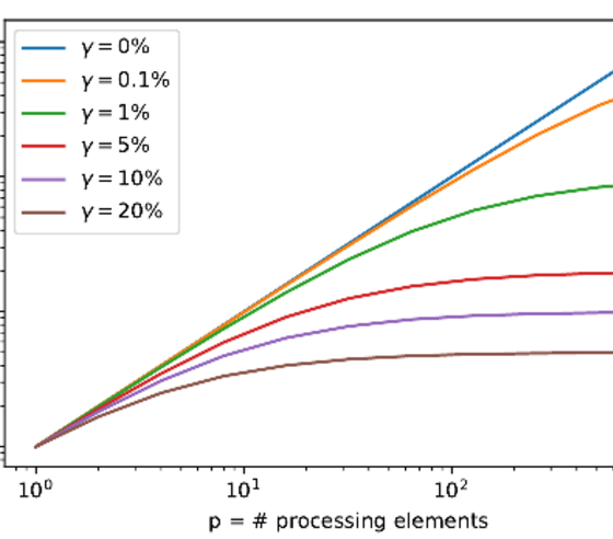
- High performance computing
- Shared memory parallelization
- Winter break
- Distributed memory parallelization
- Parallelization on graphics processing units
- Advanced CUDA by parallel reduction